A Practical RTC-Style Stitching Workaround
Stop-Gradient Guidance for Cross-Chunk Continuity
Introduction
Recent vision-language-action (VLA) models have shown impressive capability in robotic manipulation, but their high inference latency remains a major obstacle for real-time deployment. The Real-Time Chunking (RTC) framework addresses this issue by enabling asynchronous execution of action-chunked policies, reformulating real-time control as an inference-time inpainting problem. Without any retraining, RTC allows a policy to generate future action chunks while safely executing previously committed actions, achieving smooth and delay-robust behavior in both simulation and real-world robotic tasks.
While reproducing the results of this work and experimenting with its released implementation, I ran into a gradient-handling pitfall that can meaningfully affect cross-chunk continuity and runtime behavior. Specifically, when implementing RTC-style per-step “stitching” guidance, it is tempting to let gradients propagate through the learned vector field / flow policy \(v(\cdot)\) via automatic differentiation.
In retrospect, the approach described in this post is best viewed as a pragmatic workaround: it often produces an RTC-like continuity effect, but it is not necessarily a principled or faithful implementation of RTC in a strict algorithmic sense. The goal here is to document an implementation choice—stopping gradients through \(v\)—that can strengthen the guidance signal in practice, and to show what changes when you do (or do not) take that shortcut.
Preliminaries
Action chunking and horizons
RTC considers an action-chunking policy \(\pi(A_t \mid o_t)\), where
\(A_t = [a_t, a_{t+1}, \ldots, a_{t+H-1}]\) is a chunk of \(H\) future actions (the prediction horizon).
At rollout time, only the first \(s \le H\) actions are executed (the execution horizon). Longer \(s\) improves temporal consistency but reduces reactivity; shorter \(s\) increases the chance of discontinuities between chunks.
Flow policy sampling
RTC focuses on policies trained with conditional flow matching (diffusion policies can be converted to flow policies at inference time).
A chunk is generated by sampling Gaussian noise and integrating the learned velocity field \(v_\pi\) over flow time \(\tau \in [0,1)\) with \(n\) denoising steps:
Real-time constraint and inference delay
Let \(\Delta t\) be the controller period and \(\delta\) the wall-clock time to generate one chunk. RTC defines the inference delay
\[d := \left\lfloor \frac{\delta}{\Delta t} \right\rfloor, \tag{2}\]the number of control steps between receiving \(o_t\) and having \(A_t\) available. A naive asynchronous strategy can be real-time when \(d \le H - s\), but it may cause a discontinuous switch at the chunk boundary because the policy cannot predict what happens during the delay window.
RTC as inpainting with soft masking
RTC frames asynchronous chunking as an inpainting problem: while executing the previous chunk, the actions that are guaranteed to be executed due to delay are treated as “frozen,” and the rest of the new chunk is generated to be compatible with the previous one.
To strengthen cross-chunk continuity, RTC uses soft masking weights \(W\): the first \(d\) overlapping actions receive weight 1, the non-overlapping tail receives weight 0, and the intermediate region decays smoothly from 1 to 0. The guided inference step is implemented via a vector–Jacobian product (VJP) computed with reverse-mode autodifferentiation, which is exactly where gradient-handling becomes subtle in practice.
The ΠGDM Correction Term and a Stop-Gradient Approximation
In RTC, the ΠGDM-style corrected vector field can be written as
\[v_{\Pi\mathrm{GDM}}(A_t^\tau,o_t,\tau) = v(A_t^\tau,o_t,\tau) + \min\!\left( \beta,\; \frac{1-\tau}{\tau \cdot r_\tau^{2}} \right) \bigl(Y - \hat{A}_t^{1}\bigr)^\top \mathrm{diag}(W)\; \frac{\partial \hat{A}_t^{1}}{\partial A_t^\tau}, \tag{3}\]where
\[\hat{A}_t^{1}=A_t^\tau+(1-\tau)\,v(A_t^\tau,o_t,\tau). \tag{4}\]If we apply the chain rule strictly, then
\[\frac{\partial \hat{A}_t^{1}}{\partial A_t^\tau} = I + (1-\tau)\frac{\partial v(A_t^\tau,o_t,\tau)}{\partial A_t^\tau}. \tag{5}\]At first glance, it seems natural to use (5) when computing the VJP in (3).
However, if your goal is a “residual-style” stitching constraint (the inpainting/continuity view), a common practical approximation is to treat \(v\) as constant for the VJP (i.e., stop gradients through \(v\)). Under this approximation,
\[\frac{\partial \hat{A}_t^{1}}{\partial A_t^\tau} = I, \tag{6}\]and the correction direction reduces to the most direct weighted residual:
\[\min\!\left( \beta,\; \frac{1-\tau}{\tau \cdot r_\tau^{2}} \right) \bigl(Y - \hat{A}_t^{1}\bigr)^\top \mathrm{diag}(W). \tag{7}\]Why stop gradients through \(v\) in practice?
The key point is that this guidance step is trying to enforce cross-chunk continuity—conceptually an inpainting constraint that pulls the current prediction toward a target \(Y\) in the overlap region (weighted by \(W\)). In practice, letting gradients flow “through the network” can sometimes dampen the effective guidance signal, making the resulting correction term too small to meaningfully steer the trajectory at chunk boundaries. When the guidance is underpowered, the sampler largely follows the unconditional flow, and cross-chunk continuity can degrade because the constraint is not enforced strongly enough.
Here is a minimal JAX sketch of the stop-gradient workaround for 1→0 flow integration (e.g., \(\pi_{0}\)). In denoiser(), we apply jax.lax.stop_gradient(v_t) so that jax.vjp does not backpropagate through v_t_fn (i.e., treats v_t as constant w.r.t. x_t).
import jax
import jax.numpy as jnp
from typing import Callable


def pinv_corrected_velocity(
    v_t_fn: Callable, # ([ah ad], float) -> [ah ad]
    x_t: jax.Array, # [b ah ad]
    t: float,
    prefix_actions: jax.Array, # [b ah ad]
    inference_delay: int,
    prefix_attention_horizon: int,
    max_guidance_weight: float,
) -> jax.Array: # [b ah ad]
    @jax.vmap
    def _pinv_corrected_velocity(
        x_t: jax.Array, # [ah ad]
        y: jax.Array, # [ah ad]
    ) -> jax.Array: # [ah ad]
        def denoiser(x_t: jax.Array) -> tuple[jax.Array, jax.Array]:
            v_t = v_t_fn(x_t, t)
            x_0 = x_t - jax.lax.stop_gradient(v_t) * t
            return x_0, v_t

        x_0, vjp_fun, v_t = jax.vjp(denoiser, x_t, has_aux=True)
        error = (y - x_0) * get_prefix_weights(inference_delay, prefix_attention_horizon, prefix_actions.shape[1])[:, None]
        pinv_correction = vjp_fun(error)[0]
        # constants from paper
        inv_r2 = (t**2 + (1 - t) ** 2) / (t**2)
        c = jnp.nan_to_num(t / (1 - t), posinf=max_guidance_weight)
        guidance_weight = jnp.minimum(c * inv_r2, max_guidance_weight)
        return v_t - guidance_weight * pinv_correction

    return _pinv_corrected_velocity(x_t, prefix_actions)
Experiment: What does this RTC-like workaround look like in practice?
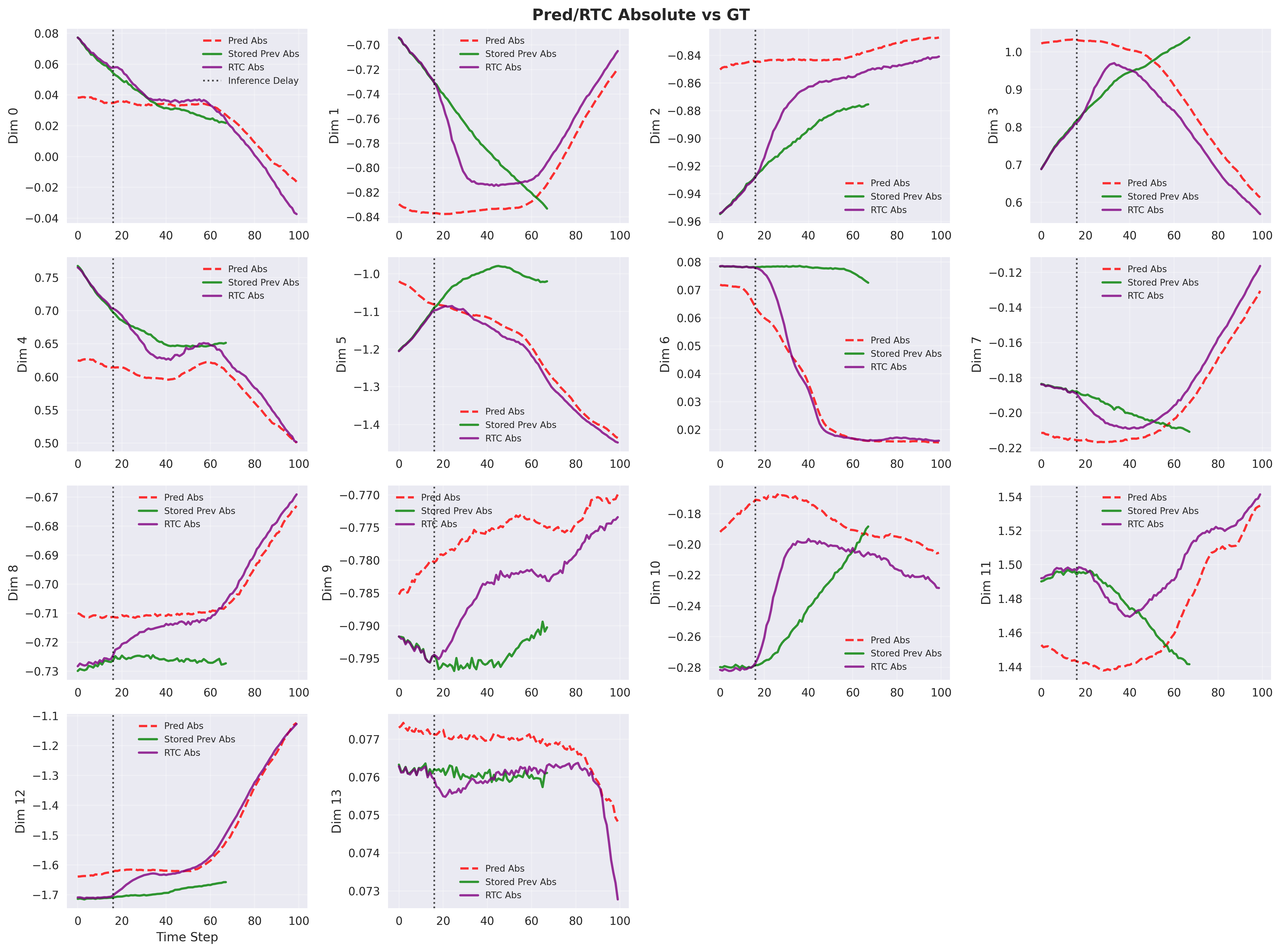
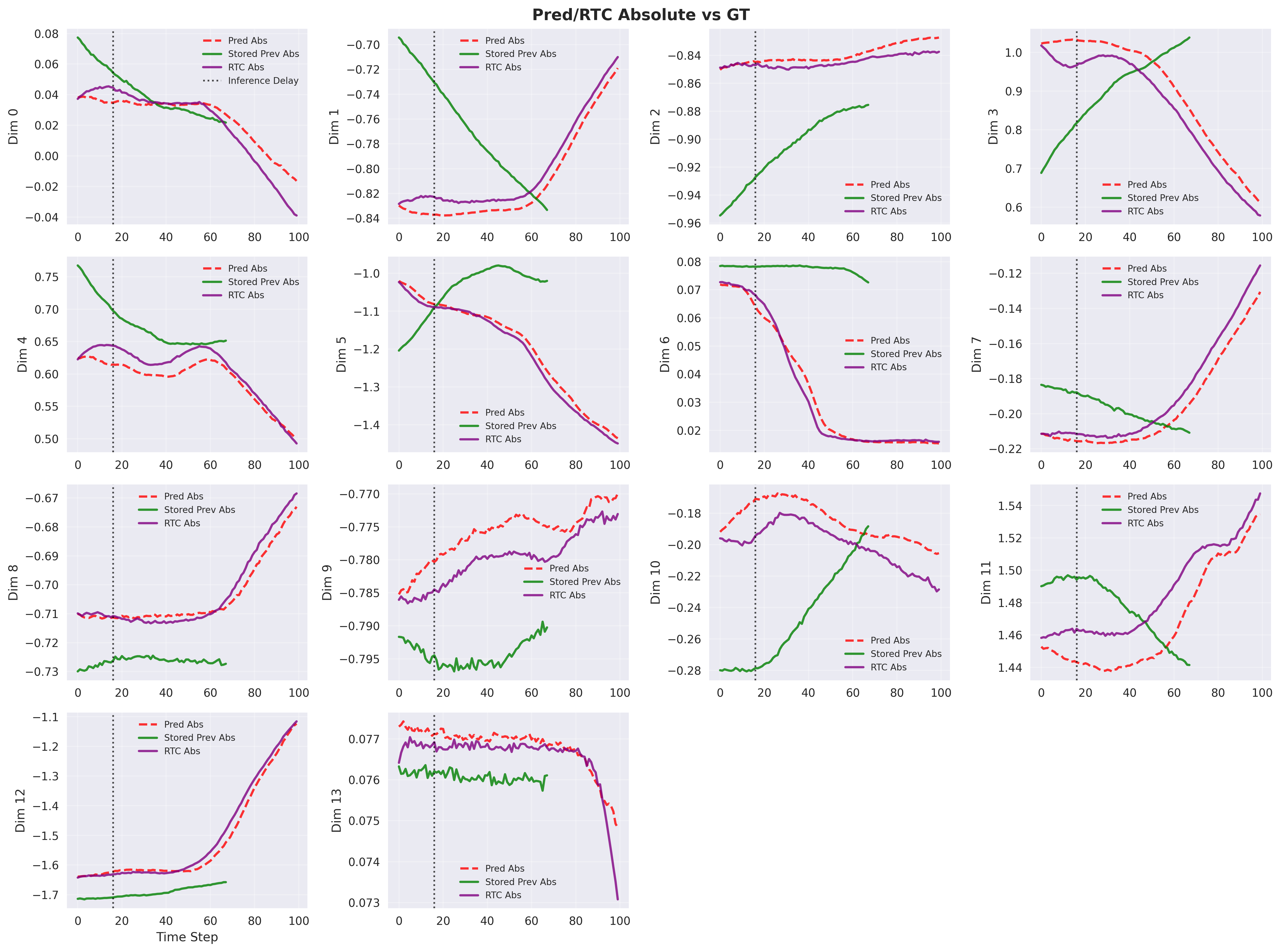
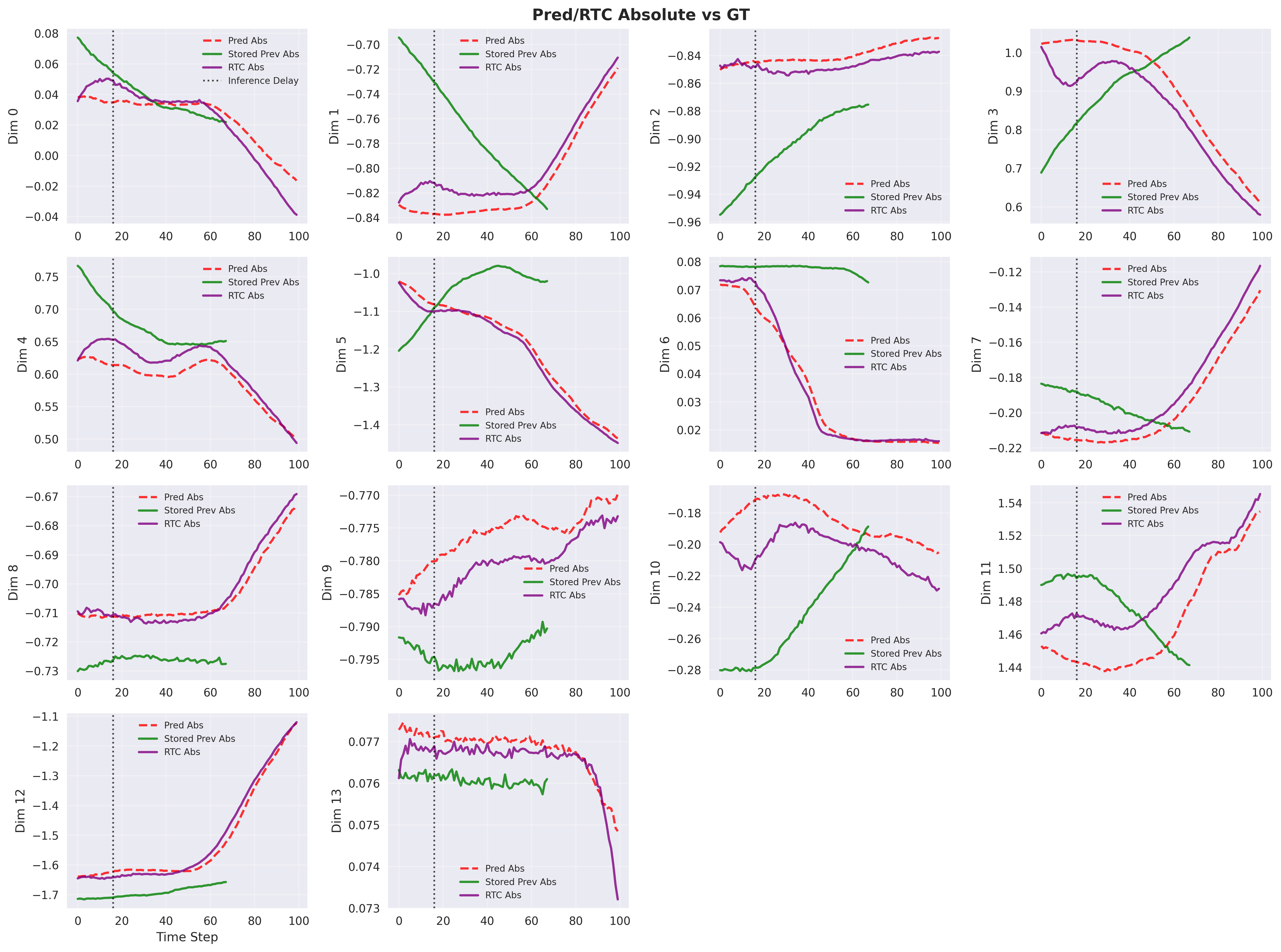
We fine-tuned \(\pi_{05}\) on a dual-arm Flexiv robot to perform a LEGO sorting task. The figure below shows results from this RTC-style stitching guidance (using the stop-gradient workaround), evaluated on dataset trajectories.
- purple denotes the actions generated with the RTC-style stitching guidance (stop-gradient workaround),
- green denotes the corresponding actions from the previous action chunk used for guidance,
- red dashed denotes the actions generated without this stitching guidance,
- gray dashed denotes the inference delay.
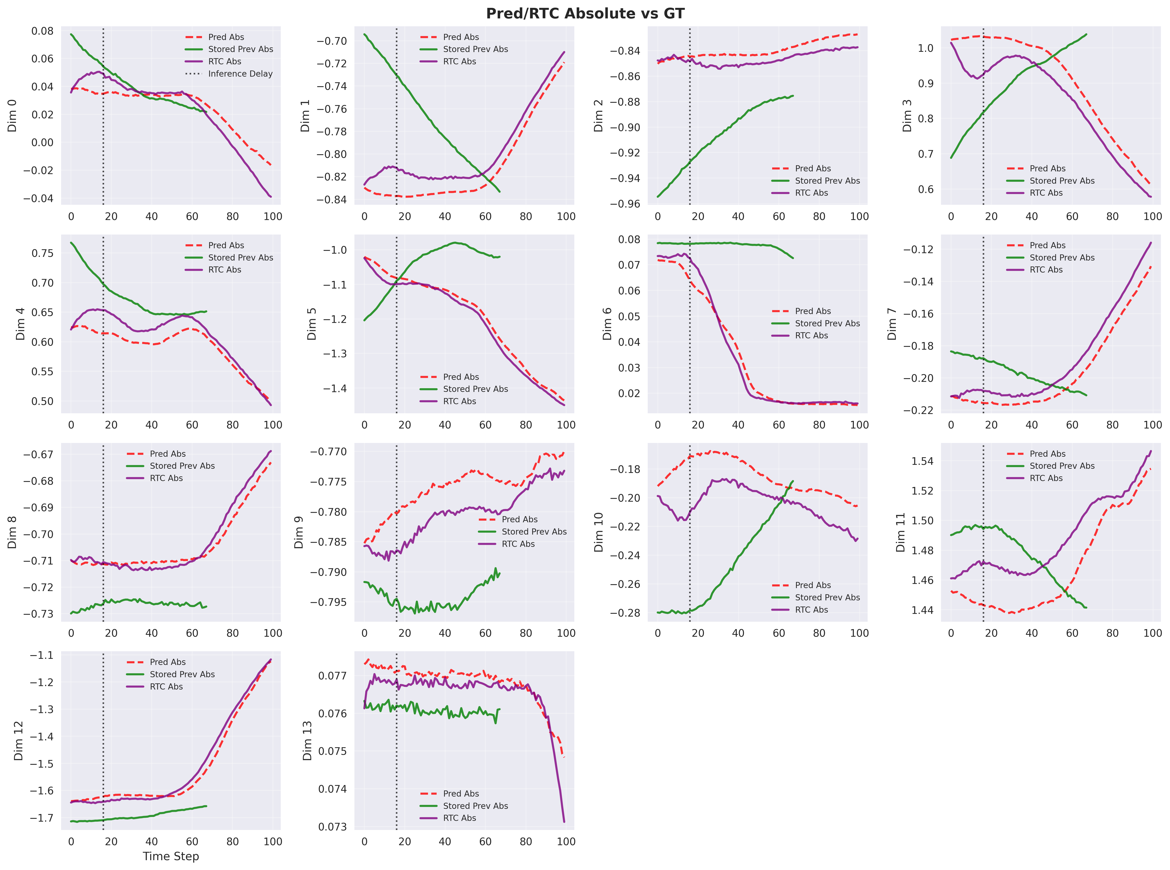
We use an action chunk length of 100. The RTC-related parameters in this test are: inference_delay = 16, max_guidance_weight = 10, and execution_horizon = 64.
Notably, the y-axis is measured in meters. The 14 dimensions in the plot correspond to \((x, y, z, r_x, r_y, r_z, \text{gripper}) \times 2\)
In contrast, using the same parameters and input data but simply removing jax.lax.stop_gradient(v_t) yields the following result:
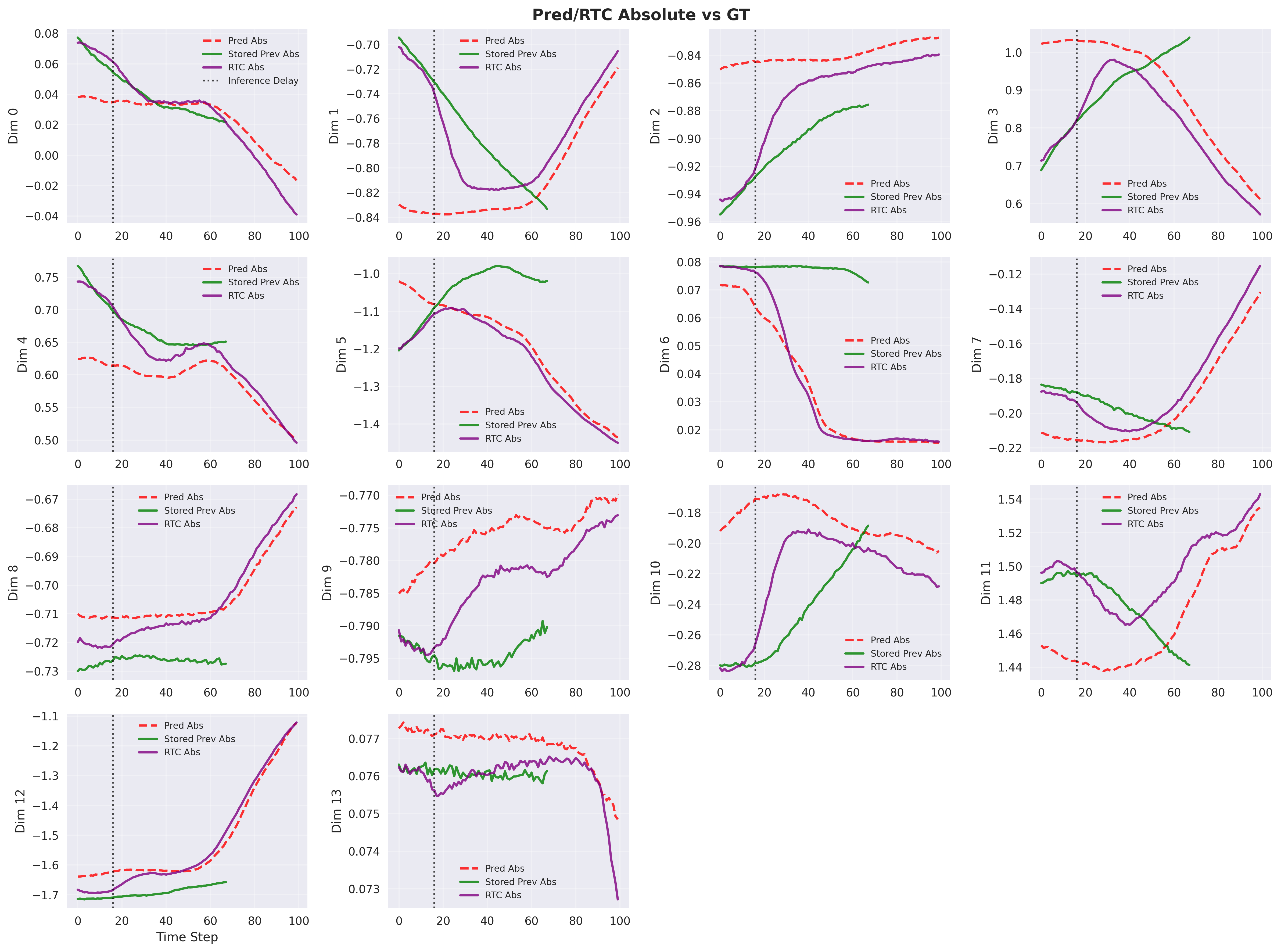
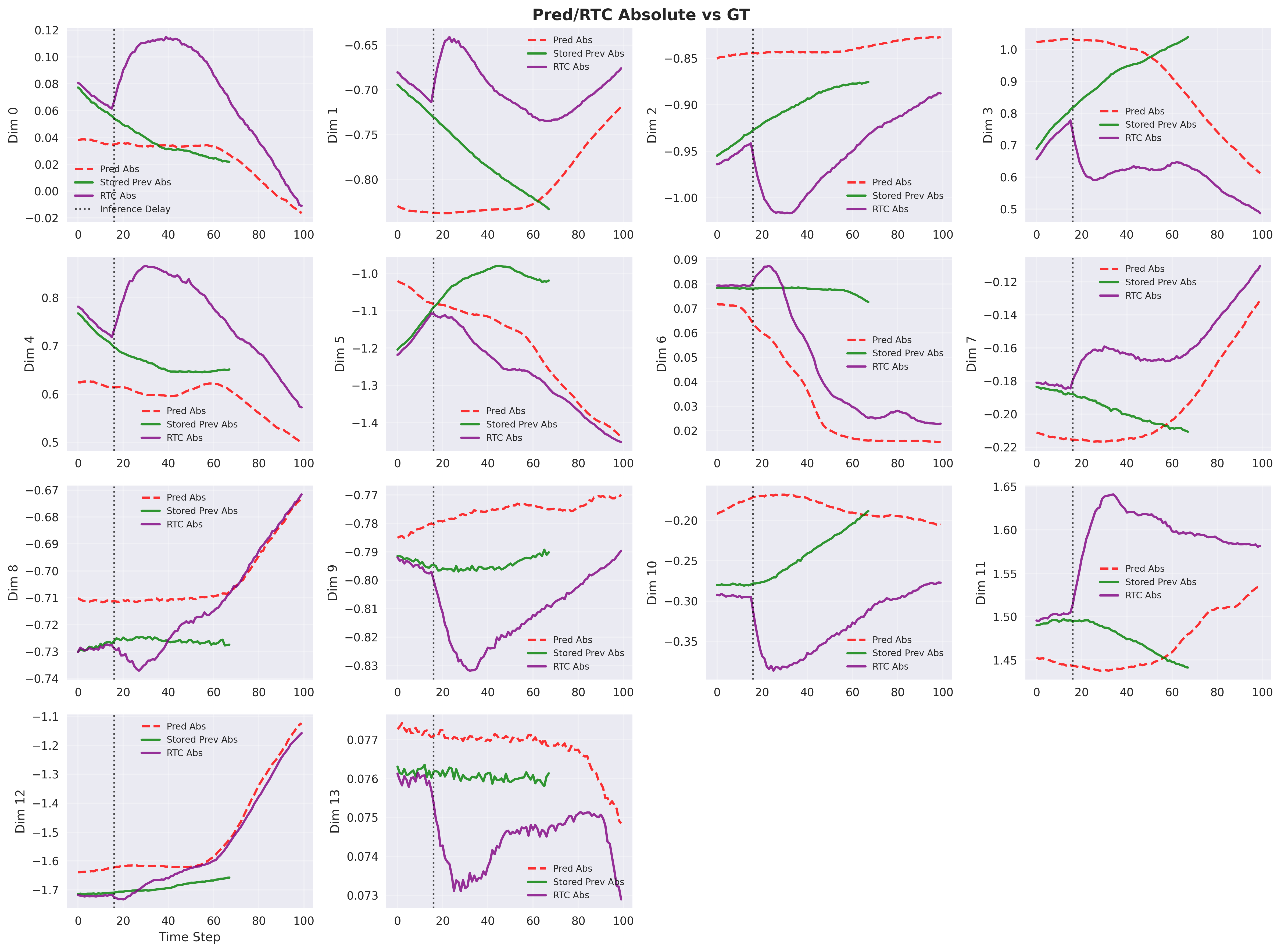
In addition, tuning max_guidance_weight suggests that max_guidance_weight = 10 is better suited for the default \(\pi_{05}\) implementation. This smoothing idea is also discussed in Soare’s blog post.1
max_guidance_weight = 5
max_guidance_weight = 100
Unmodified RTC max_guidance = 5
Unmodified RTC max_guidance = 100
⚠️ Important note / Limitations.
These experiments were conducted under fairly limited conditions—only a small number of tasks and just a handful of episodes—though we tested multiple action parameterizations, including absolute end-effector poses, relative end-effector poses, relative joint angles, and absolute joint angles. This method may encounter issues in certain scenarios, and it is only provided as a reference.
Citation
Please feel free to cite this work as
@misc{ wu2026rtc,
  author = { Linzhi Wu and Junjie Xu },
  title  = { A Practical RTC-Style Stitching Workaround },
  year   = { 2026 },
  url    = { https://xiaozhisky1.github.io/jekyll/update/2026/01/26/implementing-rtc-correctly.html },
  note   = { Blog post }
}
-
Alexander Soare, Smooth-As-Butter Robot Policies, 2025 (blog post). ↩